A_3: Fit time series | Handbook FORMAT Project

Identify, by quantitative trend analysis, how technology-related parameters have evolved in the last years.

Forecast, by quantitative trend extrapolation, how technology is going to continue its evolution in the next years.

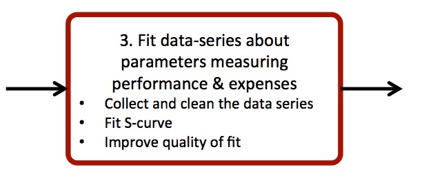
Method

Develop a quantitative trend analysis for performance and expenses. A convenient model to perform this study is the logistic growth model, largely used for technology forecasting and relatively simple to implement. The application of the model assumes that the STF follows a logistic growth; it allows identifying the variables that will limit the STF growth in the future.

Instructions

Recall the criteria to measure performance and expenses from Step 3 in Stage M.
Think about variables that can help you to understand the STFSTF = System to be forecasted and its evolution. The variables have to be meaningful for answering to the forecast question (Step 1 in Stage FOR). Consider the following:
- A number of variables have to be selected to develop the quantitative trend analysis; select what is meaningful for your STFSTF = System to be forecasted .
- Collect time data series for the selected variables from various data sources; these data sources can be internal or external.
- Order the time data series chronologically – past to present.
Develop quantitative trend analysis through suitable regression models; if the variable is likely to follow a logistic growth, perform the regression by means of one of the suggested software tools.
(for logistic growth models only) Analyse the parameters of the regression (Figure 1):
- K: the limit of growth, i.e. the maximum value that the variable can achieve in the future;
- Tm: the time of maximum annual rate of growth, i.e. the midpoint of the S-curve (Only in case when one is using yearly data);
- Δt: the time-period between the 10% and the 90% of the variable growth.
Assess the reliability of the regression by using statistical indicators. The main indicators to check are:
- R-square: R-square indicates how well data fit the regression model, i.e. it is a measure of the distance between the fitted curve and the data of the time series;
- P-value: The p-value is calculated for each parameter of the regression: a low p-value (< 0.05) indicates that the parameter is meaningful, while a larger (insignificant) p-value suggests that changes in the parameter are not associated with changes in the curve value;
Identify the evolution stage of the variable, i.e. estimate the degree of growth according to the following classification:
- Initial stage
- Growth stage
- Saturated stage
Identify the reasons or meaning of variable stage and drive some partial conclusions for the STFSTF = System to be forecasted .

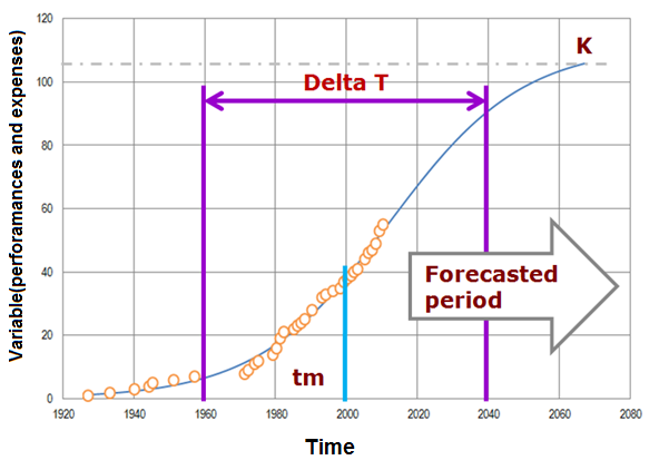
Figure1: Graphical representation of Logistic Growth Curve based on Meyer’s equation and their parameters.

Tips

➔ Before selecting the variables for forecasting, ask the beneficiaries about the availability of time data series to define the performance and expenses forecast.

➔ In order to facilitate the regression analysis, use freely available software tools (e.g. FORMAT-prototype, Loglet, IIASA LMS). The Logistics Curve Software (FORMAT-prototype) provides complete statistical information.

➔ Look for variables at different system operator levels (recall the analysis carried out in Step 5 in Stage M). Sometimes the expansion of outlook allows the extension of boundaries limiting the identification of variables showing a logistic growth behaviour.

➔ Check your results with the beneficiaries and experts in order to discuss the consistency of the regression parameters with the domain know-how and thus to derive more robust conclusions.

Example

Example -1(Washing Machine):

In a case study related to washing machine analysis, a meaningful indicator was described as “average capacity of washing machine” (US and Canada sales). Data was collected from an external database, California Energy Commission (http://www.energy.ca.gov/). Figure 2 presents the variable behaviour as fitted by a curve along with a plot of the residual error. The regression shows the data fitting with a projection for the next years. Table 1, in turn, collects the values of the regression parameters together with the statistical indicators concerning the statistical reliability of the analysis (Instruction #3 and #4).

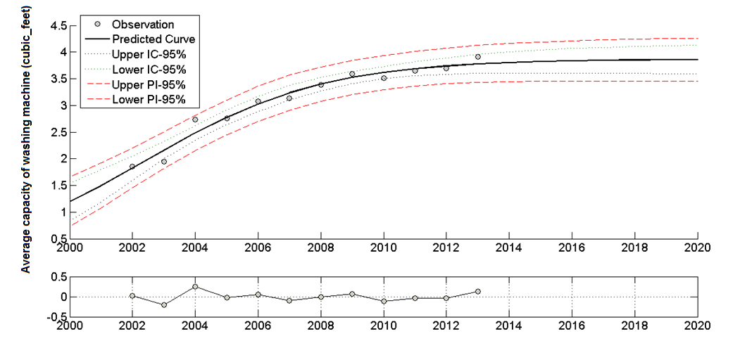
Figure 2: Average of washing machine capacity; Data source: California Energy Commission.

Table 1. Statistical results for regression analysis of washing machine capacity

Parameter	Value	Statistical significance (p)
Parameter of the regression
Maximum for average of washing machine capacity[cubic feet]	3,86 cu ft (614,47l)	p<0,01
Period of time for 80% of the cycle [years]	12 years	p<0,01
Middle time when interior volume growth achieve his 50% [years]	2002 years	p<0,01
Results of the fit
R-Squared [%]	96,83%	–

Conclusions driven by this analysis are that the average volume of washing machine in US and Canada is not going to radically change in the next years and it is highly probable that it will stabilize on a constant value (maturity stage) (instruction #5). As a consequence, it means that the next choices at the organizational level would avoid considering the idea of developing a bigger washing machine (Instruction #6).

Example -2(Copper Production):

This step was accomplished by using a performance indicator at super-system level of the grinding process. The indicator was described as “world copper production”. Data were collected from an external database, USGS mineral information and cooper worldwide. Figure 3 presents the variable behaviour as fitted by a curve along with a plot of the residual error. The regression shows the data fitting with a projection for the next years. Table 2, in turn, collects the values of the regression parameters together with the statistical indicators concerning the statistical reliability of the analysis (Instruction #3 and #4).

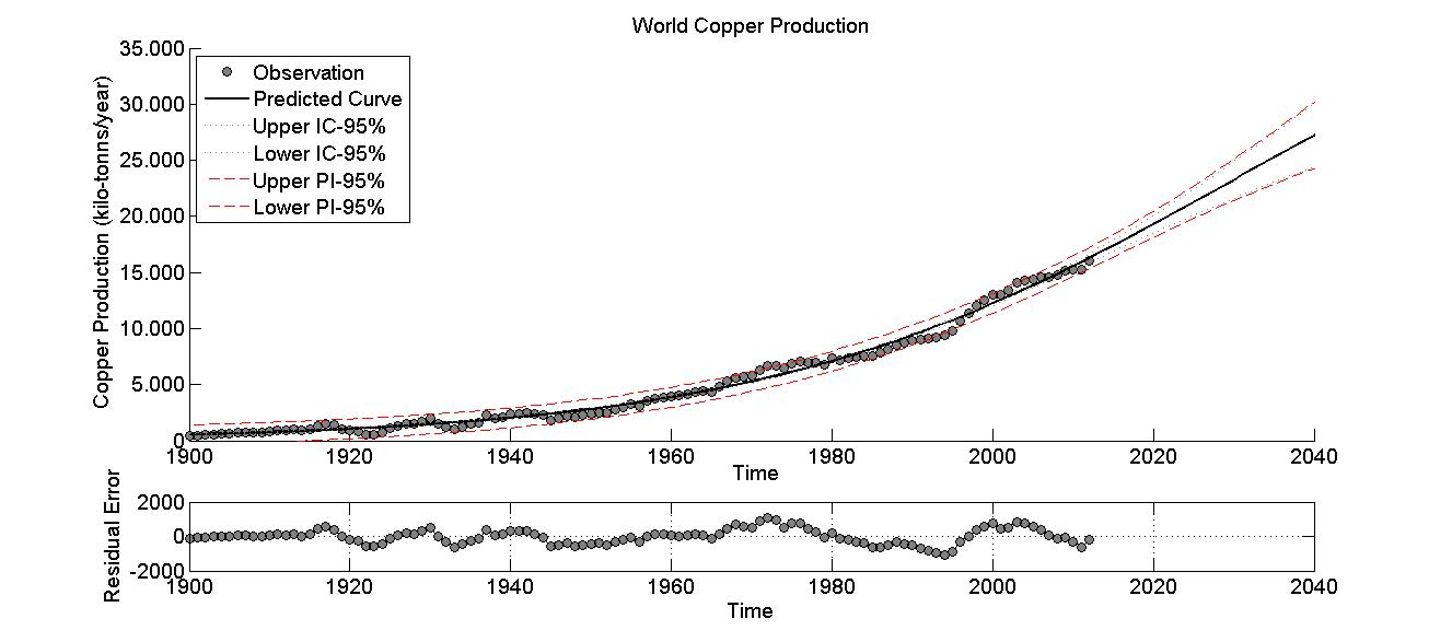
Figure 3: World copper production; Data source: USGS mineral information and cooper worldwide.

Table 2. Statistical results for regression analysis of world copper production

Parameter	Value	Statistical significance (p)
Parameter of the regression
World copper production	46836[kilo-tonns/year]	p<0,01
Period of time for 80% of the cycle [years]	128 years	p<0,01
Middle time when achieve his 50% [years]	2030 years	p<0,01
Results of the fit
R-Squared [%]	99,0%	–

Conclusions driven by this analysis are that the world copper production is going to continue increasing in the next years: it can be considered as a growing variable (instruction #5). As a consequence, it means that the R&D strategies should be focused on increasing the production according to the trend-demand. However, it should be also taken into account that the amount of copper inside the mine is decreasing, and a saturation point is expected to come (instruction #6).

v.2

← Previous step Next step →